#453 | Searching for Certainty in All the Wrong Places

Questions from astute readers answered after the article

Ask people what they want their life insurance policy to be and they’ll probably say “cheap.” That’s understandable given the bombardment every day of commercials from P&C companies advocating for folks to switch to their company in order to save a few percent on their premiums. Price competitiveness may generate a sale, but quality of coverage is literally the only thing that matters when it’s time for a claim. In P&C insurance, those two things are inextricably linked. You can’t have high quality coverage without paying for it, at least not for long.

Life insurance is a different animal. Unlike P&C, which re-trades every 6-12 months and covers a potential outcome, life insurance is a long-term contract that covers an inevitable outcome. The only thing that matters is whether or not the policy is in-force at the time of the claim. Cheap life insurance is life insurance that is less certain to pay a claim. What consumers should want, therefore, isn’t cheap life insurance – it’s certainty of coverage when the claim happens.

That’s the fundamental premise behind Whole Life. Nothing is left to chance. Premiums must be paid every year. The amount of the premium is calibrated to worst-case mortality (CSO), worst-case expenses and a guaranteed interest rate assumption that is well below expected investment returns. Guaranteed premium minus guaranteed expenses plus guaranteed interest creates a specific cash value that is hard coded into the contract itself as a tabular value. At maturity, the cash value equals the death benefit, thereby wiping out the insurance component of the contract. The inherent conservatism of the chassis and the pricing guarantees that a claim will be paid*.

The only uncertain bit about Whole Life is the dividend paid every year – but that’s by design. Only positive experience in mortality, expenses and interest flows through to the policyholder. If the policyholder elects to receive dividends in the form of Paid-Up Additions, which is almost always the case, then each dividend goes to buy a new chunk of coverage under the same guaranteed rubric. The entire Whole Life chassis is built for certainty, even the relatively uncertain parts.

All of that certainty has a cost. Because of the inherent conservatism built into the pricing, Whole Life premiums are steep. For a 55 year old Preferred male for $1M of coverage, the annual premium to age 100 is around $32,000 per year. On a guaranteed basis, therefore, the client will have paid more premiums than they’ll receive in death benefit by age 86. Is that what the client is actually going to get? Of course not. Accrued PUAs from dividends are illustrated to add nearly $1.5 million of additional death benefit by that period of time, putting the illustrated IRR on DB at around 5%. Certain premiums with uncertain future benefits is the core challenge of selling Whole Life. There’s always an element of faith, even with centuries-long track records of paying dividends.

The promise and premise of Universal Life is that it can theoretically deliver dramatically lower cost with only marginally less certainty. Is it really much of a risk, for example, to use current mortality rather than CSO? Probably not, given the historical stability of population mortality results. The same goes for policy expenses. The carrier can reliably recoup expense via fixed charges in the first 10 years of a Universal Life policy, but Whole Life assesses guaranteed premium loads for the life of the contract. The premium for a 55 year old Male for $1M of coverage using 2017 CSO mortality and a 3.75% guaranteed interest rate is around $18,750. The price quoted above is $32,000, which means that roughly 40% of the premium is expense loading.

Setting premiums in Universal Life while assuming current mortality and current expenses is a reasonable, logical approach. Both of those things are predictable and have a small range of outcomes. The likelihood of massive changes to either pricing factor is low. Whole Life may be 100% certain, but Universal Life on current expenses and current mortality with the same interest rate assumption is something like 95% certain**. There is a real argument that Whole Life – at double the premium cost – is way up on the curve of diminishing marginal returns for certainty, even if dividends ultimately refund the difference.

The problem is that Universal Life presses its advantage beyond the reliable factors of expense loading and mortality rates and into crediting rates. Consider the fact that the lowest illustrated premium on the market for the same 55 year old cell as above using an Indexed UL product at the maximum rate is a little over $11,000. That’s a little more than 1/3 of the price of a Whole Life contract and a 40% discount to the price of the “pure” Universal Life policy using the same 3.75% guaranteed rate as the Whole Life contract.

This dynamic puts a lot of weight on the crediting rate, which is inherently variable. Policy charges and expenses should change rarely, if ever. Crediting rates should change regularly, even monthly. The problem is that the variability of crediting rates isn’t obvious in the illustration. The client doesn’t get an accompanying report showing how crediting rates have changed over time. Instead, they see a static illustration in which the current crediting rate is projected to last forever. The illustration paints a picture that is the exact opposite of reality. And yet, the illustration is what producers use to calibrate the premiums that they tell their clients to pay. Everyone knows that it’s wrong. But everyone does it anyway.

The variable nature of the crediting rate combined with the goal of low premiums sets the policies up to fail. Take a look at the GIF below showing how cash values react to premium funding over time and notice the incredible, almost unbelievable sensitivity of the long-term results to minor changes in premium. I’m modeling premium here because it’s easy to do, but the effect is exactly the same for minor changes in crediting rates. Basis points in crediting rate are just dollars into the policy.

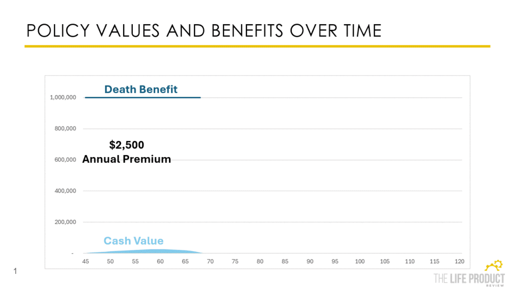
The reason is simple and I covered it in #430 | Leverage and Life Insurance. Protection-oriented sales that are designed to produce minimum premiums necessarily require lots of mortality leverage. That’s the whole point – maximum death benefit, minimum premium. But as a result, they are also necessarily the most sensitive to even slight changes in interest rates, policy charges and premium. Tiny changes will knock the entire thing out of alignment, leading to either premature lapse or over-endowment.

Think of it this way. In theory, a pencil can be stood on its head. There is a discrete point at which the center of gravity of the pencil is directly over the head and it will stand on end. And yet, it is impossible to stand a pencil on its head. Why? Because even the footstep of a ladybug or the sneeze of a gnat will knock the pencil out of perfect balance and cause it to fall. The illustration is a vacuum chamber displaying perfectly balanced pencils standing up straight every single time. But in the real world, all we see are pencils being held up or laying on the ground.

This is the defining – maybe even existential – problem in the protection-oriented end of the life insurance market that is built around the idea of offering the lowest possible premiums for lifetime coverage. Despite all of the recent press around failed premium financing and accumulation transactions, failed low-cost life insurance concepts have done vastly more harm to the industry. Vanishing premium. UL from the 1980s. VUL from the 1990s. Lifetime Guaranteed UL. Each one of those caused massive losses to either consumers or insurers. There is no such thing as cheap insurance. There is only eventual lack of coverage – or enormous risk for the insurer. You know who sold a lot of cheap life insurance? PHL Variable.

These days, cheap protection-oriented products largely exist on an Indexed UL chassis. I’ve written about these products and their unique dynamics extensively in #116, #117, #339 and #421. They illustrate low premiums, but only with enormous amounts of risk. AG 49 defaults to an aggressive illustrated rate that produces a roughly 50% chance of success even assuming S&P 500 returns of 12%, which is the historical average. Illustrating at the maximum AG 49 rate out of the box to solve for the minimum premium is setting clients up for the same scenarios that bedeviled every previous strategy to deliver “cheap” insurance. Cheap is never certain – and Indexed UL is no different.

If certainty is the goal, then we have to take a different approach. The easy choice is getting the carrier to provide certainty. Whole Life is an obvious solution. Whole Life offers the complete package of guaranteed premiums, guaranteed cash values and upside participation through dividends, but at a high price. Guaranteed UL is another option in that it offers just guaranteed premiums at a low price but forsakes cash value and upside participation. Guaranteed IUL generally offers more cash value, but no real upside participation, at least not at the minimum premium level. Guaranteed VUL can offer upside from the separate accounts, but only with high return assumptions or at high prices. Guarantees always force tradeoffs – that’s the cost of having a carrier provide certainty.

The alternative is to create certainty through the case design itself. To demonstrate how this works, I’m going to use a 55 year old Preferred Male with $1M of death benefit using Nationwide VUL Protector II. Using a 2% net illustrated rate, the level premium to endow the policy at age 100 is exactly $22,000***. The DB IRR for this policy looks like this from age 71 to 110.

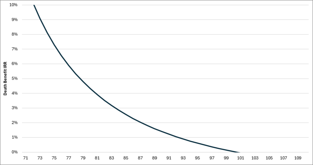
This is a classic DB IRR slope for a minimum funded design – it starts high and ends low. The death benefit remains level but the premium keeps going, so the DB IRR continues to decline. Increasing the net illustrated rate obviously drops the premium. At 4%, the premium goes to $16,561. At 6%, it drops to $12,878. And at 8%, it falls all the way to $10,644. Take a look at the effect on DB IRR:

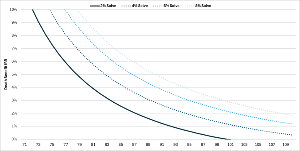
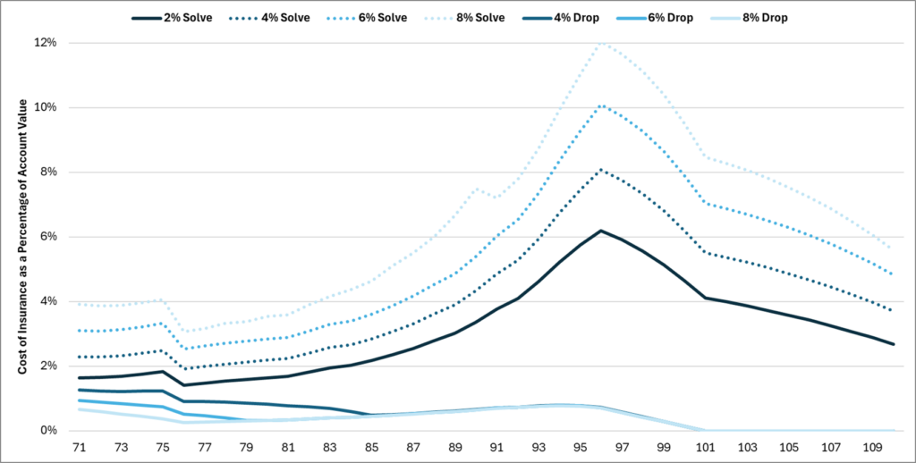
For every drop in the premium, the DB IRR increases along the same slope as the initial line using the 2% net rate assumption. However, the DB IRR increase isn’t 1-to-1 with the increase in the net illustrated rates. The rough conversion is an increase of about 0.75% in DB IRR for every 1% increase in illustrated rate after age 85. The reason is simple – COI charges. The 8% illustration has a lower premium and a lower average cash value to carry the same death benefit. As a result, it has a higher average NAR and, therefore, more COI charges as a percentage of the Account Value. In other words, the higher the illustrated rate, the lower the premium, the more drag from COIs.

You can actually see this dynamic playing out by looking at COIs as a percentage of Account Value:

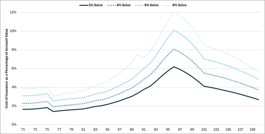
We know that illustrating higher rates results in lower premiums. We know that the higher the crediting rate, the more likely it is that the policy will underperform. That’s the natural effect of raising the bar for performance in the policy. I’m modeling VUL here because it allows for the most illustrated rate flexibility for demonstration purposes, but the effect is the same across all types of Universal Life, including Indexed UL. If you illustrate at a high rate, you increase the likelihood of underperformance.

But this graph tells the less obvious but arguably even more important part of the story. Illustrating higher rates to solve for lower premiums also magnifies COI charges as a percentage of the assets. What does that mean? More mortality leverage.More sensitivity to the underlying return assumptions. More sensitivity to natural return volatility. Illustrating higher rates of return to generate lower premiums doesn’t just create a higher hurdle rate to clear in order for the policy to work – it makes the consequences for not clearing it even more severe. It’s like adding more leverage to an even riskier bet.

This is why UL from the 1980s blew up. Those policies had a high bar to clear in terms of credited rates, but the fact that they were thin funded meant that they were levered to the hilt and collapsed quickly as credited rates fell. Variable UL from the 1990s illustrated at 12% should have been fine given that long-term equity returns were strong, but volatility killed those policies because they were mostly minimum funded. And guess what? Protection-oriented Indexed UL contracts sold at minimum premiums without secondary guarantees will suffer the same fate. If long-term index performance or lower caps don’t get them, natural crediting volatility probably will.

There is a better way. Let’s go back to the original scenario – 2% illustrated rate and a $22,000 annual premium. An alternative approach is to tell the client to pay the $22,000 but to stop paying premiums at some point in the future when and if performance exceeds 2%. It is, for lack of a better term, the Whole Life approach, but at two-thirds the cost and on a Universal Life chassis. Take a look at how these DB IRRs compare to the level premium solve DB IRRs.

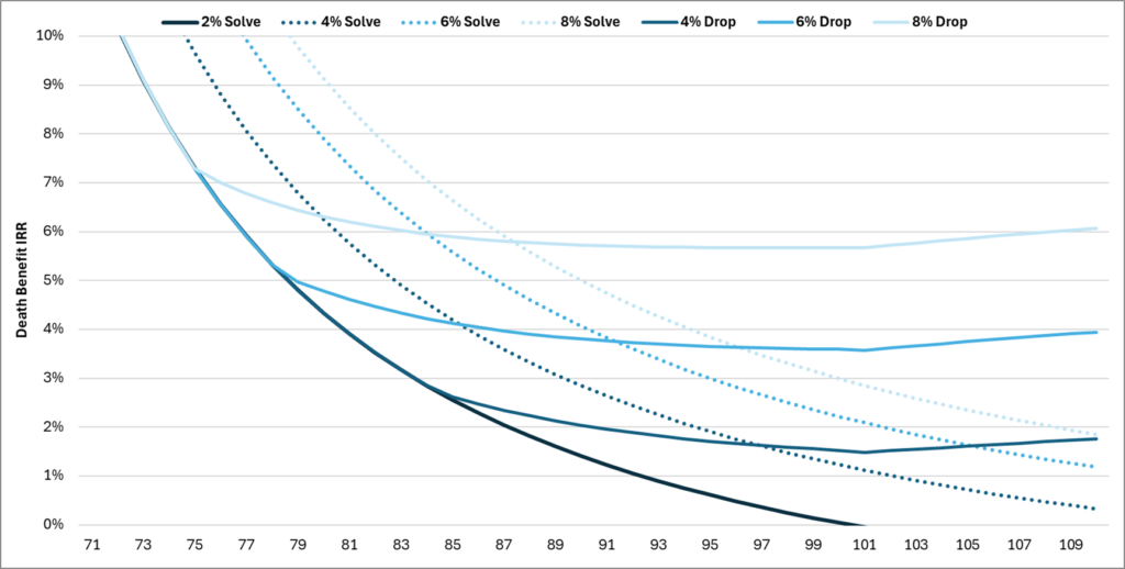
You’ll notice two things happening. First, there is an inflection point at which the DB IRR for the scenarios where performance is better than 2% break away from the 2% DB IRR line. That is the moment the policy hits CVAT corridor****. Several magical things happen in that moment all at once. The first is that the carrier should stop taking your premiums anyway because additional premiums will increase NAR.

The second is that the DB becomes purely a function of the Account Value. Mortality leverage is now controlled by the corridor factor. As a result, COI charges as a percentage of Account Value are always the same regardless of underlying Account Value performance. A policy with $5 million of AV and a policy with $500k of AV that are both in corridor for the same client in the same year will have the same death benefit as a percentage of the AV, which means they’ll also have the same COI as a percentage of the AV. It doesn’t matter if one started with $1 and other started with $1 million.

Third, as you can see from the graph above, the difference in DB IRRs now matches almost perfectly with the change in the credited rate. Going from a 6% net illustrated rate to an 8% net illustrated rate increases the DB IRR by a little more than 2% over time. Why is that? Because it’s the inverse of the minimum funded scenario. The influence of COIs actually lessens as the illustrated rate increases because the policy has been overfunded, not minimum funded. Paying more early and waiting for higher performance to come later de-risks and de-levers the policy.

You can see both phenomena playing out in the charts showing COIs as a percentage of AV. The better the policy performs, the lower the drag from COI charges. Once a policy is in corridor, it has the exact same COI as a percentage of AV as all other policies in corridor. It’s magical.

There are profound implications for case design. Take a look at the chart showing DB IRRs and you’ll notice that the break-even point for DB IRRs – as in, the point at which the drop funded DB IRR exceeds the premium solve DB IRR – gets younger and younger as policy performance increases. Why is that? Because COI drag works in opposite directions in the two designs. Higher performance results in more COI drag for premium solve scenarios, but less COI drag for the drop funded scenarios. At 4%, the breakeven is age 97. At 6%, it’s 92. At 8%, it’s just age 87. At 10%, it falls to just 83. This is a no-brainer. Only in the worst-case return scenarios would the client be better off with minimum funding.

To say nothing of the inherent risk. Getting it wrong in the drop funded scenarios just means a few more premiums. A 2% net return obviously requires lifetime premium payments, but 4% allows the client to stop paying premiums at age 85. At 8%, that drops to age 75. Either way, the core characteristics of the policy are preserved and coverage is maintained. Getting it wrong in the premium solve scenarios means a policy lapse and huge future costs to keep the policy going. Using the 8% premium solve but actually getting 4% causes a policy lapse at age 89 and requires a $90,000 premium to keep the policy going to age 100.

In short, you can pay the carrier to create certainty through guarantees – or you can create certainty by changing the case design to start with a higher premium that stops once the policy hits corridor. It’s an unbundled version of Whole Life with premium flexibility and participation in upside performance. Whole Life is the embodiment of certainty and consistency of behavior. That’s not because Whole Life is special. It’s because Whole Life lives in the CVAT corridor. Any and all policies in the CVAT corridor will exhibit the same certainty and consistency of behavior as soon as they get there too. CVAT corridor turns a wolf into a show dog, behaving perfectly and predictably on command.

The predictability of policy performance when funded to reach CVAT corridor essentially eliminates risk from the policy itself as the underlying Account Value changes. If the Account Value drops, then the death benefit drops and NAR contracts. If the AV increases, then DB increases and NAR expands. The policy only takes on more NAR when it can handle the increase. This is completely the opposite of the behavior in a minimally funded policy where falling AV expands NAR and therefore increases COI, creating more drag on policy performance. There is no doom spiral when the policy is in CVAT corridor, but there is if the policy has been minimally funded and misses the mark.

Certainty in the policy itself allows for greater uncertainty about asset returns. In short – you can take more risk in a policy that has been funded conservatively than you can in a policy that has been minimum funded because the policy can handle it. Policies that are minimally funded need to constantly manage for both long-term returns and short-term volatility, which is one reason why the default for most insurance professionals is to recommend fixed and indexed insurance contracts and eschew variable contracts.

Policies that are funded to reach CVAT corridor have none of the same restrictions. They are concerned with long-term returns only to the extent that they exceed the conservative baseline. Short-term volatility has no effect on the relationship between policy charges and the Account Value. You can throw literally any return sequence at the policy and as long as it stays in corridor, it behaves exactly the same way. Blow an airhorn and the show dog will not flinch.

As a result, it’s reasonable to allocate much more aggressively in policies with higher funding than policies with minimum funding. You can do Variable UL without being afraid of volatility wrecking the policy. It might be reasonable, for example, to even go all equities when a policy is heading towards corridor. If that’s the case, then the comparisons above that assume the same returns from the same assumed allocations regardless of how the policy is funded aren’t realistic. Policies funded with higher premiums should also get more aggressive allocations with higher average returns. If you assume the drop funded scenarios earn 2% more on average than the minimum funded scenarios, the breakeven year is just age 85. That’s a young buck in the world of life insurance.

This view is an inversion of the typical approach to policy selection. Producers go for fixed insurance policies with low return volatility because they assume those are safer for protection-oriented sales. In doing so, they’ve set themselves up for a scenario where they’ve eliminated all short-term volatility – a near necessity for minimum funding – but they’ve also surrendered any real potential for long-term outperformance. In the best case, they’ll get bond-like returns. In the worst case, they’ll be stuck in a moribund portfolio at a life insurer no longer interested in writing new business that hammers guaranteed rates to the absolute minimum and never relents.

But in all cases, they have absolutely no control. The long-term performance of every fixed policy is at the complete mercy of the company issuing it. That is by far the greatest risk to any policyholder – just ask folks at PHL Variable, Accordia, Security Life of Denver and even Lincoln, which dropped crediting rates on its entire in-force block to the guarantees and still hasn’t brought them back to market levels despite rising asset returns. No amount of proper planning or funding can offset a carrier intent on draining value from its in-force block.

The alternative is to use Variable UL. Producers have eschewed it because of the perceived risk of the chassis – but that perception was borne from underfunded policies in the 1990s. Properly funded VUL is the least risky Universal Life variant. It allows for complete control of the investments, including fixed and indexed options in most policies. Unlike other types of UL, there is actual return history for the asset classes that allow for reliable expectations of future returns. If the policy is at or near corridor, asset returns flow right through without changing the product characteristics. Short of Whole Life, properly funded VUL is the most predictable, most understandable and most stable product the life insurance industry has to offer.

Consumers say they want cheap policies – because they presume that all policies are equally certain to pay claims. That presumption is false. Cheap policies are always less certain. Creating certainty costs something. If the life insurer creates certainty, it comes with high fixed premiums or benefit tradeoffs. If we can create certainty through smart case design, then we can have our cake and eat it, too. Flexible premiums. Upside participation. Predictable policy behavior. The capacity to take asset risk. Certainty, but on the policyholder’s terms and in their control. Certainty that’s worth paying for.

*The only way a claim wouldn’t be paid is if the carrier had asset losses that blew through capital and surplus. But even then, some percentage of the claim would still be paid.

**I know carriers have changed COIs and expenses – I’ve written about it at length – but the vast majority of carriers haven’t. And even in the scenarios where some charge structures were changed, the changes were often applied to only a small subset of the overall block. In my view, UL policy charge structures are generally reliable.

***Ok, fine. It’s $21,999. On sale!

****Yes, you should always set these policies up as CVAT. And yes, I know CVAT isn’t technically a corridor, but it is a corridor for contractual purposes and clients can see it in their policy documents.

Question – What about GPT?
Answer – The same core concept applies, but you’d have to contend with the Guideline Level Premium limitation, which could get in the way for certain products and funding scenarios, particularly shorter premium solves. To get around that, you need to use an Option 2/B/Increasing DB during the premium payment period, which creates excess NAR that would need to be fixed with a future face decrease. Overall, it just isn’t as clean and, therefore, I recommend sticking with CVAT. You’ll never regret having a bit more death benefit along the way, but the client’s beneficiaries could definitely regret an untimely face amount decrease.

Question – Aren’t there scenarios when a declining AV could actually expand NAR?
Answer – Yes, absolutely. The article is built around the idea of the policy being in one of two states – in CVAT corridor or out of it. Reality isn’t so black-and-white. Until AV grows to a multiple of the original face amount, there’s a possibility that a steep decline in the AV from investment losses (in a VUL) could push the AV to the point where the policy stops being in corridor. A similar effect could happen once you start taking withdrawals. If you want to maintain the minimum amount of coverage, then you just need to monitor whether the policy is in or out of corridor. But if you’re more concerned with keeping the contract inforce no matter what, then ask for the face amount to be reduced to the minimum after the policy is safely in corridor after year 7. It won’t trigger any material modification – at least, that’s my understanding – because there is no change to the current policy values but it will ensure that the policy stays in corridor even if the AV drops until, of course, the minimum face amount prevails.

Question – How should I set this up for a case design?
Answer – Keep it simple. CVAT. Option 1/A/Level death benefit. Solve for premium to endow at a conservative rate that you think is achievable 95% of the time, something like 2-3%. That’s it!