
This version of the article was made available to LISA for limited use at their request. Otherwise, it is meant to be for Subscribers to The Life Product Review only. Please do not distribute this link. If you’d like to sign up for The Life Product Review and read the other 359 articles, click here.
Risk is a fiendishly difficult thing to quantify. In financial theory, risk is usually quantified in terms of standard deviation – the greater the variance, the greater the risk. Famously, Nassim Taleb popularized the idea of “black swan” events that don’t fit into a nice and neat normal distribution but are a regular feature of distributions with “fat tails.” The fact that the Great Financial Crisis was often described as a multi-sigma event says more about the quality of the risk model than it does about the event itself. As a result, financial risk is increasingly being seen less in terms of tame volatility and more in terms of ruin, fragility, convexity and asymmetry, all of which are non-linear and unpredictable.
If risk is hard to define and quantify in traditional financial instruments, it is even more so for life insurance. There are just too many elements – mortality experience, policy funding, non-guaranteed element changes, life insurer investment returns, non-linear policy charges, just to name a few. A “risky” product can be made safe by appropriate funding. A “safe” product can be made risky by inadequate funding. A “solid” product can come undone by changes to non-guaranteed charges. A “well-funded” product can lapse if crediting performance deteriorates.
That is why there has never been a comprehensive philosophy, framework or model for risk in life insurance products. I’ve been asked many, many times over the years to come up with some sort of “scoring” system for life insurance products to quantify their risk and return potential and my answer every time is the same – it’s impossible. In my view, there is no way to do it and to support it with a broadly applied and rigorous framework that isn’t riddled with exceptions.
Because real risk quantification is essentially impossible, the industry seems to fall back on a simplified view of risk based on pure volatility of returns. We assume that Whole Life is riskless because the cash value is guaranteed to grow and the death benefit is guaranteed to be in-force. We assume that Universal Life has slightly more risk because it has weaker guarantees. We assume that Indexed UL has still more risk because it has variability of index-linked returns, despite having a crediting floor. And we assume that Variable UL has still the most risk because it can experience the full ups and downs of the market, full volatility. When you do that, you get a “risk spectrum” that usually is stylized to look something like this:
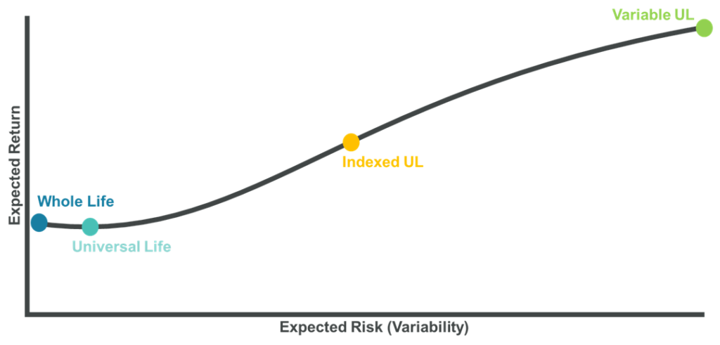
As I wrote in #135 | Indexed UL on the Risk Spectrum – Part 1, this sort of middle-ground positioning for Indexed UL is not correct. In reality, by any statistical measure of variance, “risk” in Indexed UL is virtually indistinguishable from risk in Universal Life. A more accurate graph would have Indexed UL nearly overlapping with Universal Life.
The positioning for Variable UL is also incorrect. VUL can have fixed accounts, indexed accounts, structured accounts and separate accounts that range from money market funds to small cap tech funds. The reality is that VUL covers nearly the whole spectrum. That’s what makes it such a powerful product. And finally, the reason why I put Whole Life above Universal Life is because of participation. Some long-term returns in Universal Life will have to go to shareholders. But with participating products, those long-term returns only have one place to go – policyholders. As a result, all else being equal, participating Whole Life should outperform non-participating Universal Life.
However, I think this sort of risk/return analysis is fundamentally misleading for the simple reason that all of the returns on this graph, with the exception of Variable UL returns in separate accounts, are discretionary. The life insurer controls them. Whole Life should outperform Universal Life, but if the company writing the Whole Life policy has issues – as we saw with Ohio National – then the relationship could invert. Same goes for Indexed UL versus Universal Life if the company pummels caps for in-force policyholders, as Accordia has done.
And, of course, Universal Life can perform significantly worse than Whole Life if the company drops the crediting rate to the guarantees and refuses to increase them even if conditions have improved, which is what Lincoln did in 2011 to its in-force Universal Life block and has kept them there ever since. This graph only works if all of the products are written and priced identically by the same life insurer. Other than that, all bets are off. These dots could be anywhere.
As a result, I would argue that we need a fundamentally different way of looking at risk in life insurance. We need to isolate the risk down to the actual product structure, not its expected return by asking a different question – assuming returns are X and the product is funded to Y, how much variability will there be in the actual result? In other words, we need to assume that proper company selection takes out the issue of performance differentials and, instead, focus on what the product actually does and how it works relative to the original expectation.
For Whole Life, the answer is pretty simple – there isn’t any risk. If credited returns are X and policy funding is Y, then you know both the guaranteed and non-guaranteed values. As you move X around between low and high, the non-guaranteed values will change, with the worst-case scenario being the guaranteed values. But even more importantly, any value of X that produces dividends that buy Paid-Up Additions means that those PUAs are now added to the guarantees. In other words, the worst-case scenario improves as X increases.
The same can’t be said for Universal Life. Like Whole Life, knowing credited returns are X and policy funding is Y means that you also know how the policy will perform, but low X values can still cause policy lapse due to charges, which isn’t a possibility in Whole Life. Furthermore, guarantees in Universal Life are usually nowhere near as strong as in Whole Life, which means that the worst case scenario is quite a bit worse than in Whole Life. The tradeoff, of course, is flexibility. But that’s not a part of this analysis.
For Indexed UL, the answer is very different. The carrier declares a Cap (in this example), not a credited rate, so X is always an assumption about how the Cap translates into the performance of the policy. AG 49/A/B dictates that the maximum illustrated rate, which is usually taken as the default assumption for policy performance, is predicated on a three step process. First, apply the current Cap to historical index returns. Second, calculate the 25-year geometric return average for each trading day for the past 66 years. Third, calculate the arithmetic average of the 25-year geometric averages. Voila. That’s the maximum AG 49/A/B illustrated rate.
As I’ve written about before at length, this process creates a return assumption that is actually pretty aggressive. It uses historical index returns that are substantially higher than the expectation for future index returns provided by major managers and, in my experience, far higher than financial planners use for projections for planning purposes. It applies the currently declared Cap without consideration to whether the Cap is sustainable or reasonable. But most egregiously, it takes the average which, as I’ve shown before, sits at around the 55th percentile mark, meaning that 45% of the 25 year periods actually would have performed worse than the maximum illustrated rate. Illustrating at the maximum AG 49/A/B rate bakes in a high risk of underperformance. However, that’s not the topic of this article.
Let’s just assume for a moment that we know, beyond the shadow of a doubt, that a Cap set at Z will produce illustrated performance of X. Regardless of whether X is 4%, 6% or 8%, there is another factor at play that doesn’t get enough attention – the interaction between the fundamentally variable nature of index-linked returns and the policy charges, which is often referred to as dollar “sequence of return risk.” This risk is impossible to model using life insurance illustrations because we can’t show any return in any year in excess of AG 49/A/B. As a result, it doesn’t get discussed except in general terms and it is never quantified. At least, until now.
Enter Life Insurance Sustainability Analytics (LISA), an independent website that models Indexed UL and Variable UL products using a rigorous statistical methodology targeted explicitly to quantifying the effects of dollar sequence of return risk. The secret sauce for LISA, in my opinion, is the fact that it can run anywhere from a single dollar return sequence to a thousand dollar sequences of returns through a policy chassis that all have the exact same average return and standard deviation. LISA is essentially built to answer the question we’re asking – assuming that we know the crediting performance is X and policy funding is Y, then how will the policy perform? And I have to admit, the answers shocked me.
First, some background. For this analysis, I used the four free pre-loaded LISA demonstration samples that model generic Indexed UL and Variable UL products that are based on actual product offerings. I did some replication of the numbers on the website and, in my view, they’re representative of what you’d get in a typical retail product. The accumulation sample in LISA uses a 20-pay premium and a stream of income from years 21 to 40 and that’s what I used. For protection sample, LISA pays a minimum level premium for 20 years. It can be extended but I stuck with 20 years because I didn’t think it would change the output enough to bother with changing the sample.
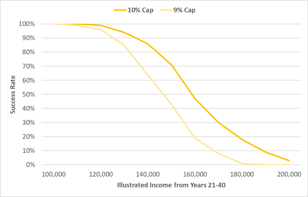
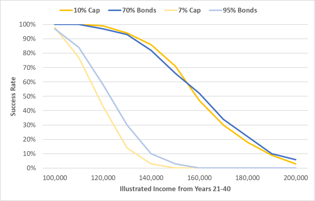
I started with the Indexed UL accumulation sample and started messing around with the model in a very simple way. The basic illustration has a $159,000 annual loan distribution using an (old) Indexed UL product illustrated at 6.09% based on a 10% Cap. After a bit of recalibration to get the model to spit out 6.09% average returns for each scenario, the failure rate is 50%. To put that into words, what LISA is saying is that even if the average return is the same 6.09% as in the level rate illustration, 50% of the 1,000 scenarios would have lapsed prior to age 100 with the illustrated income stream. Those failures are not due to poor performance because every scenario has the same average return. Those failures are due specifically to poor dollar sequence of returns.
This is a shocking finding. What it shows is that Indexed UL is incredibly, almost unbelievably, fragile. What would it take to get the probability of failure down to zero? A drop in illustrated income from $159,000 to around $118,000, a 26% reduction in illustrated income just to overcome the dollar sequence of return risk. If you graph out the probability of success by illustrated income, here’s what it looks like for both a 10% Cap and 9% Cap.
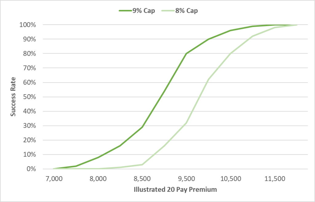
A similar phenomenon occurs for thin-funded, protection-oriented sales, but the chart looks different. As the premium falls, so does the success rate. The premium would have to increase by around 35% to take out dollar sequence of return risk. Take a look:
Let me put this in blunt terms. What LISA shows is that if you are illustrating at the maximum AG 49/A/B rate, then you are illustrating a 50% failure rate even if you are right about the long-term average return*. In order to take dollar sequence of return risk out of the equation and therefore put Indexed UL on a level playing field with Universal Life and Whole Life, neither of which have the same sort of sequence of return risk, then you would need to do a 25% decrease in illustrated income for a distribution sale or a 35% increase in illustrated premium for a protection sale.
In my experience, very few agents bake conservatism into their Indexed UL illustrations. Most run it at the maximum AG 49/A/B rate and tell the client that the calculation itself is conservative, which is demonstrably false. The agents who do reduce the illustrated rate generally do it because they think that the maximum illustrated rate is aggressive relative to long-term expectations. That may be true, but it’s a different line of reasoning than what I’m addressing here. The issue at hand is not long-term averages. All of this analysis assumes that the long-term average is actually in-line with AG 49/A/B. The risk we’re addressing is purely due to dollar sequence of returns. That means that every single Indexed UL illustration needs a 25-35% haircut just to counteract dollar sequence of return risk. That is a stunning, jaw-dropping, paradigm-shifting revelation that should fundamentally change the way that everyone illustrates Indexed UL.
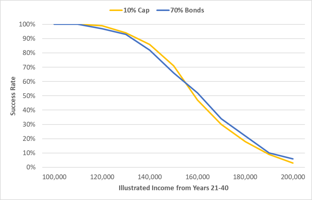
Now, what about Variable UL? This one also held some surprises. LISA allows for a sliding scale of equity and bond exposure. Blending 70% fixed income and 30% equities yields a very, very similar result to an Indexed UL with a 10% Cap. Take a look:
At first blush, this is a compelling argument in favor of Indexed UL and its ability to replicate a portfolio of bonds and stocks. But there is a big wrinkle in the story. The equity allocation is closely correlated to the Cap level. The higher the Cap, the larger the equity allocation to produce a similar result. So the key question here is the appropriate Cap level for the purposes of this model to ensure that the Cap is consistent with the underlying assumptions. In LISA, equities are pegged at an 11.04% average return with a 16.79% standard deviation. Fixed income is pegged at 3.53% with a standard deviation of 4.62%. The average return and standard deviation of the equities and fixed income benchmarks are derived from 20 years of rolling monthly annual returns.
Taking the LISA fixed income yield as a reasonable proxy for a new money crediting rate, at least within the confines of this analysis, a 10% Cap is way out of bounds. There is no way that a life insurer could afford a 10% Cap with a 3.53% option budget. Instead, the Cap would be more like 7% based on today’s option prices. To replicate close to the probabilities of success for a 7% Cap, you’d need something more like 95% bonds and 5% equities, and even that portfolio beats Indexed UL. See below.
I mentioned earlier that Indexed UL has very nearly the same risk profile, from a statistical standpoint, as Universal Life. Therefore, it should have very nearly the same performance – which is exactly what LISA shows. Based on LISA’s data, which uses an equity assumption in excess of 11%, Indexed UL at fair market rates essentially replicates a 95% bond and 5% equity portfolio. In other words, it assumes that the long-term return on the options portion of the strategy is about the same as long-term equity returns, not 45% like in the AG 49/A/B construct. Hard to argue with that logic.
And, it bears repeating, these assumptions use an 11.04% average equity return. If you really think equities are going to rip at 11.04%, then you should be in Variable UL. The knock on VUL is always that there is a “double-whammy” effect where volatility creates higher policy charges due to expanding NAR and that will sink the product. As intuitive as this logic is, it doesn’t apply to fully funded, accumulation-oriented Variable UL sales. Now look at the exact same analytics as the Indexed UL products above, but this time with a 100% equity allocation:
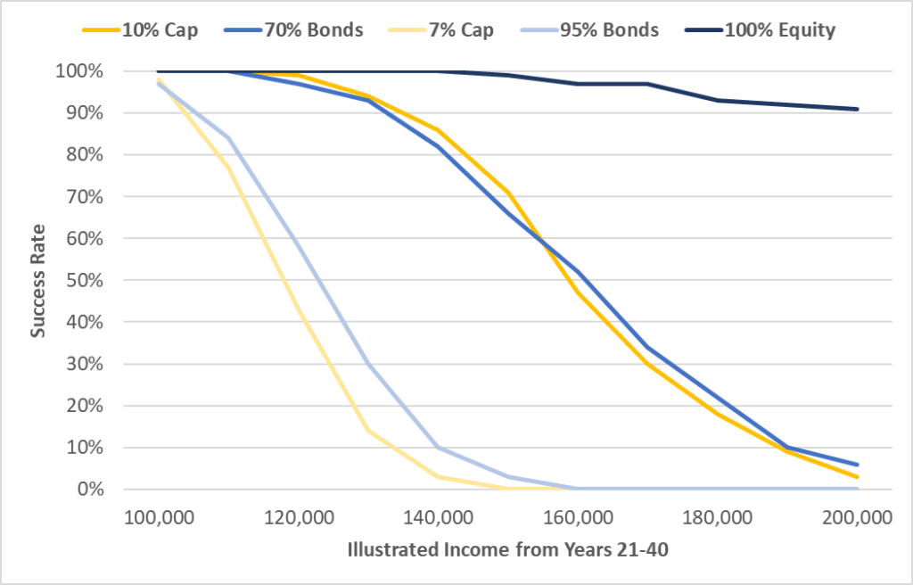
What these results show is that if you buy into the assumptions underpinning the analysis – which are shared by both Indexed UL and Variable UL models – then illustrating $200,000 of income out of VUL has a 90% success rate compared to about 3% for Indexed UL with a 10% Cap and 0% for Indexed UL with a fair-market (as defined by LISA parameters) 7% Cap.
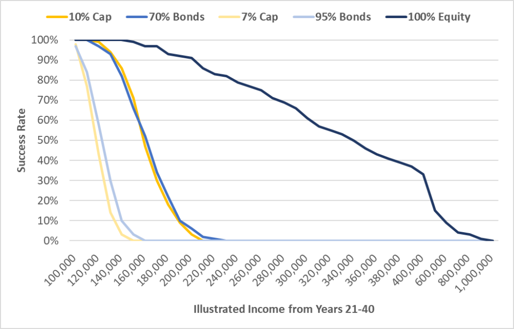
In other words, volatility itself doesn’t sink Variable UL. For the same level of income, Variable UL is actually much safer than Indexed UL, despite the fact that Variable UL has much higher levels of volatility. This is counterintuitive but sit with it long enough and it will start to make sense. Both products have variability. The difference is that even though the variability is higher in Variable UL, the actual risk of failure is much lower for the exact same dollar result for the client because the returns are so much higher. With the same underlying equity assumptions as Indexed UL, Variable UL premiums can generally be 35% lower or, with accumulation scenarios, VUL can have income that is double the results of Indexed UL with the same probability of success. And what if you were willing to take a much lower probability of success? Here is the same graph as above, but this time extended all the way out to $1 million in annual income:
The same sort of phenomenon also manifests in thinly-funded, protection-oriented sales, but with a bit of a twist. In these sorts of sales, policy performance is much more sensitive to sequence of returns because of the expanding NAR issue. The “double whammy” effect has some teeth. Take a look at the same chart as earlier, but this time with a 100% Equities allocation in a VUL:
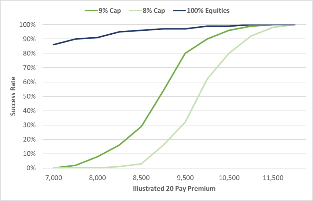
If the goal is 0% dollar sequence of return risk, then the funding level is about the same between IUL with a 9% Cap and Variable UL with 100% equities. With an 8% Cap assumption, then Variable UL is cheaper. And, of course, if the client is willing to take (say) 10% risk from dollar sequence of returns, then Variable UL prices in at $7,500 against $10,000 for Indexed UL with a 10% Cap. LISA makes a compelling case for using VUL, even for thinly-funded, protection-oriented scenarios.
However, there’s a caveat. If equity returns perform at 7%, for example, with the same 16% standard deviation, then the gap between Indexed UL and Variable UL may narrow, depending on how the returns materialize. Indexed UL is more sensitive to the way the returns materialize than the average return itself. For example, equities could have a 0% average return but with a lot of consistent increases punctuated by a few steep declines and Indexed UL would outperform pure equities. We can’t know that sort of thing. But LISA provides a reasonable baseline.
In my view, LISA is the most powerful and insightful tool into Indexed UL and Variable UL product performance that I’ve ever seen. It is thoughtfully created and incredibly well executed. Beyond the samples that I’ve used for this analysis, users can subscribe in order to run an unlimited number of illustration benchmarks. This would money well spent, to be sure, but the rules of thumb using the benchmarks are clear: Haircut Indexed UL illustrations by 25-35% even if you think you’re right about the long-term average return. With the same underlying equity assumptions, Variable UL can deliver premiums that are 35% lower or income that is double the results in Indexed UL with the same level of success.
I used to joke that “Indexed UL is the El Camino of life insurance. Part car, part truck, doesn’t do either particularly well.” It’s funny. It gets a good laugh. But there’s some truth to it. Like the El Camino, Indexed UL has no compromises on paper. But in the real world, there are more compelling alternatives. If you really want downside protection, Whole Life is a superior chassis. If you really want upside potential, Variable UL will blow the doors off of Indexed UL.
However, that doesn’t mean Indexed UL is without a place. Fundamentally, Indexed UL is a psychological sale. It’s downside protection with upside potential. Clients love that story. It resonates with the fear-over-greed part of our brains. There is a powerful behavioral finance angle. And in certain situations, Indexed UL can substantially outperform Universal Life and Whole Life, as we saw over the past decade when equities were ripping, options were cheap and portfolio yields were high. I remain a fan of the product. I absolutely see the utility and I think index-linked crediting deserves a place in nearly every company’s product portfolio. But we need to get real about how the inherent risk of the chassis and how it should be illustrated against other products. Normal illustrations can’t do that, but LISA can, and that’s the power of the platform.
*LISA doesn’t do AG 49/A/B replication out of the box. The regulation uses a very specific way of calculating lookback returns that isn’t really applicable anywhere else, and certainly not for modeling equity and bond returns. As a result, if you run LISA, you’ll notice that the returns modeled for Indexed UL are usually 20-30bps lower than the AG 49/A/B maximum illustrated rate, which pushes the probability of success down to around 35%. To counteract that effect, I increased the participation rate used in LISA up to the point where the average in LISA exactly matched the AG 49/A/B average, which yielded around a 50% success rate.
Life Insurance Sustainability Analytics is an independent firm. I have no ownership stake, revenue interest or business relationship with LISA. I was shown a demo of LISA last year and took 8 months or so to get around to digging into the statistical model to really understand what it was doing and to see how to use it. But once I did, I immediately realized the power of what they’d built and how it could provide insight in ways that other tools can’t. Here’s what LISA gave me to provide as information about the service:
Life Insurance Sustainability Analytics (LISA) is an online subscription-based service that tests the “likelihood of success” for expectations created by Indexed and Variable UL Illustrations. Underpinning LISA is a stochastic engine (sometimes referred to as Monte Carlo analysis) that interpolates hundreds of “dollar sequence of returns” to demonstrate the probability of success of the illustrated policy sustaining to age 100.
LISA was developed by Michael Lockitch, CFA (CEO and Founder of Life Insurance Analytics) and has its origins in the Historic Volatility Calculator (developed by Dick Weber of The Ethical Edge) – an earlier exploration of life insurance illustration volatility testing. LISA is currently relied upon by consultants, financial planners, insurance agents and agencies to provide critical analysis and policy insights to corporate boards, trustees, and individuals for new policy design and in-force management of life insurance policies.
Access LISA here: LifeInsuranceAnalytics.com